Even with the latest advancements in ETL/ELT tools, data engineers still deal with data that arrives late or out of order which can wreak havoc on dimensional data models. Over the years I’ve dealt with this scenario more times than I can count and have had to build pipelines to handle recovery which usually required resetting the SCD2 and batch reloading data to ensure proper data order in the tables. Imagine my excitement when I found Snowflake dynamic tables and how using them can eliminate the need to reload all of my source data to guarantee a properly aligned SCD2 table from source data.
In the following demo, I’ll walk through a real scenario I faced as part of a data engineering team where we built a SCD2 table for customer data from a well-known CRM system. The full scenario details have been modified/simplified to protect the guilty innocent, but still explain the difficulty we faced with properly loading the data from the CRM.
The CRM system would deliver JSON Files in batches where every record would include the customer’s unique ID in the CRM system and a timestamp field indicating when the record was changed. The files could contain one or many customer records and would only contain changed fields in addition to the customer ID and timestamp. This setup made managing changes to customer records difficult in a traditional SCD2 setup because when we loaded the JSON, if only one field was updated, the rest of our staging table would populate as NULL since we didn’t have a value for each element.
At the time I encountered this scenario, I was working with SQL Server and at the time, the only path forward we had was to build rather complicated stored procs to compare the inbound records to the current record in our SCD2 to determine deltas on the record. You can imagine how difficult this would be if files arrived late or accidentally processed out of order – even with timestamps in the data.
Snowflake’s Dynamic Tables makes managing this scenario a breeze. Using out-of-the box processes, functions and objects, I’ll handle both the late arriving/out-of-order data issue and NULL values of the delta files. The end result being an SCD2 with proper start and end date without having to reset or batch reload any data.
Let’s dive in to the demo. All the code and sample files are available in my GitHub Repo.
Environment Setup
First, let’s setup our Snowflake environment. In the script below, we’ll create a dedicated role, warehouse, and database, as well as schemas for our bronze, silver and gold layers. In the scripts below, I drop the PUBLIC schema which is created by default in Snowflake. It’s personal preference, but I typically drop it and create dedicated schemas as needed for my projects. Lastly, we’ll create a stage and file format which will assist in loading our JSON files.
USE ROLE ACCOUNTADMIN;

--======================================
-- VARIABLE DECLARATION
--======================================
SET CUR_USER = CURRENT_USER();
SET ROLE_NAME = 'DEMO_SCD_ROLE';
SET WH_NAME ='DEMO_SCD_XS_WH';
SET DB_NAME = 'DEMO_SCD_DB';

--======================================
-- SETUP DEDICATED ROLE FOR QS
--======================================

USE ROLE SECURITYADMIN;
CREATE OR REPLACE ROLE IDENTIFIER($ROLE_NAME);
GRANT ROLE IDENTIFIER($ROLE_NAME) TO ROLE SYSADMIN;
GRANT ROLE IDENTIFIER($ROLE_NAME) TO USER IDENTIFIER($CUR_USER);

--======================================
-- SETUP DEDICATED WAREHOUSE
--======================================
USE ROLE SYSADMIN;
/*CREATE XS WORK WAREHOUSE*/
CREATE OR REPLACE WAREHOUSE IDENTIFIER($WH_NAME)
    WAREHOUSE_SIZE = XSMALL
    MIN_CLUSTER_COUNT = 1
    MAX_CLUSTER_COUNT = 1
    AUTO_SUSPEND = 300
    AUTO_RESUME = TRUE;
GRANT OWNERSHIP ON WAREHOUSE IDENTIFIER($WH_NAME)
    TO ROLE IDENTIFIER($ROLE_NAME);

--======================================
-- SETUP DEDICATED DATABASE
--======================================
USE ROLE SYSADMIN;
CREATE OR REPLACE DATABASE IDENTIFIER($DB_NAME);
USE DATABASE IDENTIFIER($DB_NAME);
GRANT OWNERSHIP ON DATABASE IDENTIFIER($DB_NAME)
    TO ROLE IDENTIFIER($ROLE_NAME);
USE ROLE IDENTIFIER($ROLE_NAME);
USE DATABASE IDENTIFIER($DB_NAME);


--======================================
-- SETUP SCHEMAS
--======================================
USE ROLE IDENTIFIER($ROLE_NAME);
USE SCHEMA INFORMATION_SCHEMA;
CREATE OR REPLACE SCHEMA BRONZE;
CREATE OR REPLACE SCHEMA SILVER;
CREATE OR REPLACE SCHEMA GOLD;
DROP SCHEMA IF EXISTS PUBLIC;

--======================================
-- SETUP STAGE AND FILE FORMAT
--======================================
USE ROLE IDENTIFIER($ROLE_NAME);
USE DATABASE IDENTIFIER($DB_NAME);
USE SCHEMA BRONZE;

/*CREATE STAGE FOR LANDING FILES*/
CREATE OR REPLACE STAGE RAW_JSON_STG
    DIRECTORY = (ENABLE=TRUE)
    ENCRYPTION = (TYPE='SNOWFLAKE_SSE');

/*CREATE THE FILE FORMAT*/
CREATE OR REPLACE FILE FORMAT JSON_FMT
    TYPE = JSON,
    COMPRESSION = AUTO;
Bronze Layer – Raw File Ingestion
Before creating the bronze layer tables, upload the raw JSON files to the stage created above. The files are numbered 01, 02 and 03 – indicating the order in which the data was updated. This will also make it easier to load them out of order to showcase how dynamic tables can make this scenario much easier to manage.
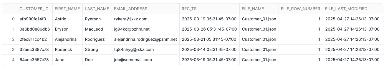
We’ll take advantage of Snowflake’s VARIANT data type to load the contents of the JSON directly to a Snowflake table, and then use JSON functions and query syntax to parse the data as needed. Additionally, we’ll use METADATA functions to capture items such as file name, row number, file last modified date and the load date in the raw table. The script below will create the table and load the first customer file from the stage created above.
USE ROLE DEMO_SCD_ROLE;
USE SCHEMA DEMO_SCD_DB.BRONZE;


CREATE OR REPLACE TABLE CUSTOMER_JSON_RAW (
	RAW_JSON VARIANT,
	FILE_NAME STRING,
	FILE_ROW_NUMBER NUMBER(38,0),
	FILE_LAST_MODIFIED TIMESTAMP_TZ(9),
	FILE_LOAD_DT TIMESTAMP_TZ(9)
);

COPY INTO BRONZE.CUSTOMER_JSON_RAW(
    RAW_JSON
    ,FILE_NAME
    ,FILE_ROW_NUMBER
    ,FILE_LAST_MODIFIED
    ,FILE_LOAD_DT
)
FROM
    (SELECT
        $1
        ,METADATA$FILENAME
        ,METADATA$FILE_ROW_NUMBER
        ,METADATA$FILE_LAST_MODIFIED
        ,METADATA$START_SCAN_TIME
    FROM
        @BRONZE.RAW_JSON_STG)
FILE_FORMAT = (FORMAT_NAME = 'BRONZE.JSON_FMT')
FILES = ('Customer_01.json');

Parse JSON with Dynamic Table
For our first dynamic table, we’ll flatten the JSON loaded above into the individual columns needed for further processing in the pipeline. In this example, we’re setting our TARGET_LAG to DOWNSTREAM since this table will be used as part of a pipeline with other dynamic tables.
The DOWNSTREAM keyword will cause this dynamic table to refresh only when a table downstream of it requires a refresh. For this example, that will be our GOLD layer current view table that we’ll create shortly. Also, I set the INITIALIZE as ON_CREATE so that the table will populate as soon as I create it and I can review the output immediately.
USE ROLE DEMO_SCD_ROLE;
USE SCHEMA DEMO_SCD_DB.BRONZE;

CREATE OR REPLACE DYNAMIC TABLE BRONZE.CUSTOMER_RAW
    WAREHOUSE = DEMO_SCD_XS_WH
    TARGET_LAG = DOWNSTREAM
    INITIALIZE = ON_CREATE
AS
    SELECT
        J.VALUE:"cid"::STRING AS CUSTOMER_ID
       ,J.VALUE:"fname"::STRING AS FIRST_NAME
       ,J.VALUE:"lname"::STRING AS LAST_NAME
       ,J.VALUE:"email"::STRING AS EMAIL_ADDRESS
       ,TO_TIMESTAMP_TZ(J.VALUE:"ts"::NUMBER,3) AS REC_TS
       ,R.FILE_NAME
       ,R.FILE_ROW_NUMBER
       ,R.FILE_LAST_MODIFIED
       ,R.FILE_LOAD_DT
    FROM BRONZE.CUSTOMER_JSON_RAW AS R,
        LATERAL FLATTEN(INPUT=>R.RAW_JSON) AS J;
Silver SCD2 Dynamic Table
Next, we’ll create the SCD2 dynamic table from the RAW table we just created. Notice that the raw data indicates the record timestamp (REC_TS), we’ll use that field to sort the raw data and use the LAG window function over the CUSTOMER_ID, which is the unique identifier, to set the end date on the SCD2.
USE SCHEMA SILVER;

CREATE OR REPLACE DYNAMIC TABLE CUSTOMER_SCD
    WAREHOUSE = DEMO_SCD_XS_WH
    TARGET_LAG = DOWNSTREAM
    INITIALIZE = ON_CREATE
AS
    SELECT
        CUSTOMER_ID,
        FIRST_NAME,
        LAST_NAME,
        EMAIL_ADDRESS,
        REC_TS AS START_DATE,
        LAG(REC_TS) OVER (PARTITION BY CUSTOMER_ID ORDER BY REC_TS DESC) AS END_DATE,
        FILE_NAME,
        FILE_LOAD_DT
    FROM
        BRONZE.CUSTOMER_RAW;
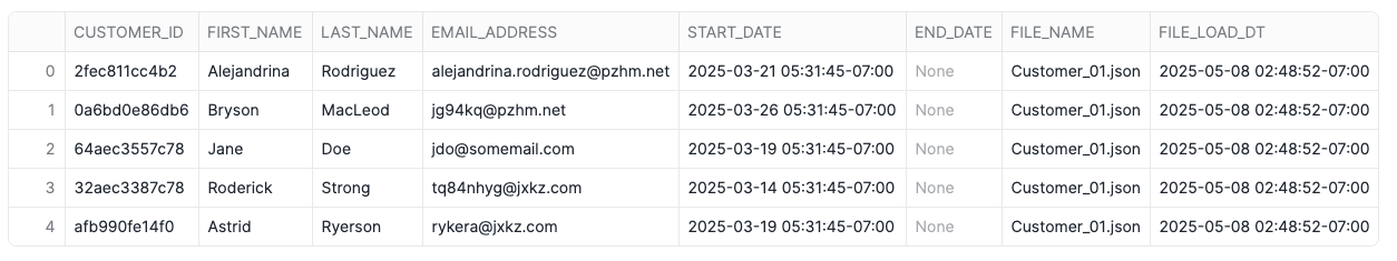
Notice that the END_DATE is NULL indicating that these are the current records. If necessary, we can add the COALESCE function around the LAG function to help set END_DATE to a default future value.
Out Of Order File Load
Next, we’ll load customer file 3 to simulate and out of order file load. After loading, we’ll manually refresh the SCD Dynamic Table which will then also refresh the RAW table since we’re setting up a Dynamic Table pipeline. Snowflake manages the dependencies automatically and begins to create a Dynamic Table DAG to manage the refreshes.
COPY INTO BRONZE.CUSTOMER_JSON_RAW(
    RAW_JSON
    ,FILE_NAME
    ,FILE_ROW_NUMBER
    ,FILE_LAST_MODIFIED
    ,FILE_LOAD_DT
)
FROM
    (SELECT
        $1
        ,METADATA$FILENAME
        ,METADATA$FILE_ROW_NUMBER
        ,METADATA$FILE_LAST_MODIFIED
        ,METADATA$START_SCAN_TIME
    FROM
        @BRONZE.RAW_JSON_STG)
FILE_FORMAT = (FORMAT_NAME = 'BRONZE.JSON_FMT')
FILES = ('Customer_03.json');


ALTER DYNAMIC TABLE SILVER.CUSTOMER_SCD REFRESH;
SELECT * FROM SILVER.CUSTOMER_SCD ORDER BY CUSTOMER_ID,END_DATE DESC;
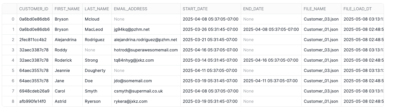
Take a look at the first two records above. The dynamic table set the end date of record from Customer_01.json properly and a new record from Customer_03.json is now “active”; however, the email address isn’t populated any longer. There are some other instances of NULL values in columns where the prior record is populuated. Let’s take a look at the source files to see if this is correct.
/*CUSTOMER_01.JSON*/
{
"cid": "0a6bd0e86db6",
"email": "jg94kq@pzhm.net",
"fname": "Bryson",
"lname": "MacLeod",
"ts": 1742992305822
}
/*CUSTOMER_03.JSON*/
{
"cid": "0a6bd0e86db6",
"fname": "Bryson",
"lname": "Mcloud",
"ts": 1744115825554
}Notice that in the second file, fname and lname both were included. There was only a change lname and email was omitted, indicating no change. The SCD dynamic table properly reflects what the raw data shows; however, that isn’t quite what the plan was as we’ve now lost the email address in the current record. Enter a new window function – FIRST_VALUE which will return the first value of a column based upon a partition and sorting window. In this case, we’ll use the same partition and sort value as our LAG function for END_DATE which will return the first value in the data for the most recent active record in the SCD.
FIRST_VALUE also allows for a bounding window on the search, when left unbounded, the function searches all rows in the partition in the order specified. By using the bounding clause, we can set for the window of rows to consider relative to the current row. In this example, I’ve set the window start at the current row and look at all trailing rows. Additionally, I’ve paired it with a COALESCE to that if the current record is populated, the SCD will use that value; otherwise, it will look for the first non-NULL value.
USE SCHEMA SILVER;

CREATE OR REPLACE DYNAMIC TABLE CUSTOMER_SCD
    WAREHOUSE = DEMO_SCD_XS_WH
    TARGET_LAG = DOWNSTREAM
    INITIALIZE = ON_CREATE
AS
    SELECT
        CUSTOMER_ID,
        COALESCE(FIRST_NAME,FIRST_VALUE(FIRST_NAME)
            IGNORE NULLS OVER (PARTITION BY CUSTOMER_ID ORDER BY REC_TS DESC
            ROWS BETWEEN CURRENT ROW AND UNBOUNDED FOLLOWING)) AS FIRST_NAME,
        COALESCE(LAST_NAME,FIRST_VALUE(LAST_NAME)
            IGNORE NULLS OVER (PARTITION BY CUSTOMER_ID ORDER BY REC_TS DESC
            ROWS BETWEEN CURRENT ROW AND UNBOUNDED FOLLOWING)) AS LAST_NAME,
        COALESCE(EMAIL_ADDRESS,FIRST_VALUE(EMAIL_ADDRESS)
            IGNORE NULLS OVER (PARTITION BY CUSTOMER_ID ORDER BY REC_TS DESC
            ROWS BETWEEN CURRENT ROW AND UNBOUNDED FOLLOWING)) AS EMAIL_ADDRESS,
        REC_TS AS START_DATE,
        LAG(REC_TS) OVER (PARTITION BY CUSTOMER_ID ORDER BY REC_TS DESC) AS END_DATE,
        FILE_NAME,
        FILE_LOAD_DT
    FROM
        BRONZE.CUSTOMER_RAW;
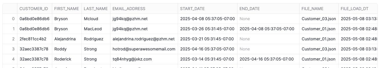
Late Arriving File
With the SCD dynamic table loading properly based on the first two files loaded, let’s see what happens when a late arriving file is loaded. Customer_02.json contains a record update for Bryson Mcloud that occurred between the timestamps of Customer_01.json and Customer_03.json – which in a typical loading pattern would require the engineering team to reset the SCD to a point in time and then load the files in proper order. Let’s see how the dynamic table handles this.
COPY INTO BRONZE.CUSTOMER_JSON_RAW(
    RAW_JSON
    ,FILE_NAME
    ,FILE_ROW_NUMBER
    ,FILE_LAST_MODIFIED
    ,FILE_LOAD_DT
)
FROM
    (SELECT
        $1
        ,METADATA$FILENAME
        ,METADATA$FILE_ROW_NUMBER
        ,METADATA$FILE_LAST_MODIFIED
        ,METADATA$START_SCAN_TIME
    FROM
        @BRONZE.RAW_JSON_STG)
FILE_FORMAT = (FORMAT_NAME = 'BRONZE.JSON_FMT')
FILES = ('Customer_02.json');

ALTER DYNAMIC TABLE SILVER.CUSTOMER_SCD REFRESH;
SELECT * FROM SILVER.CUSTOMER_SCD ORDER BY CUSTOMER_ID,END_DATE DESC;
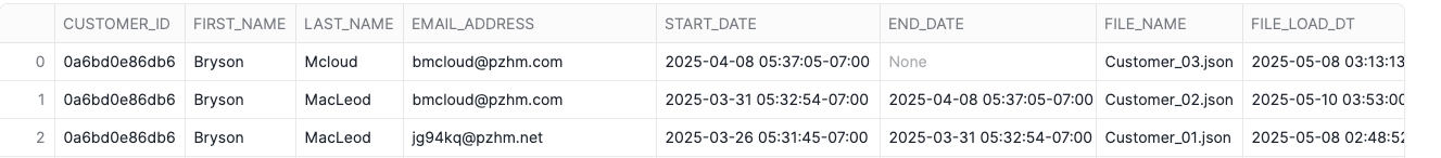
Notice that the SCD2 properly “healed” itself by placing the record from Customer_02.json in the right time order. Also notice that the files were loaded two days apart, further confirming that the dynamic table can handle very late arriving data!
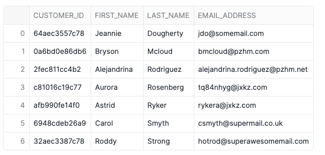
Active “Driver” Dynamic Table
Lastly, we’ll setup our gold layer active view of the SCD for use in reporting or dashboards, etc. We’ll do this with a dynamic table as well, but since this table will serve as “the end of the pipeline”, it’ll refresh on a set interval rather than when a downstream table needs it. For the gold layer, I’ve excluded the start and end dates as well as the file information. This is entirely optional; however, it showcases how dynamic tables can use almost any SQL query as the source.
CREATE OR REPLACE DYNAMIC TABLE GOLD.CUSTOMER
    INITIALIZE = ON_CREATE
    TARGET_LAG = '1 MINUTE'
    WAREHOUSE = DEMO_SCD_XS_WH
AS
    SELECT
        * EXCLUDE (START_DATE,END_DATE,FILE_NAME,FILE_LOAD_DT)
    FROM
        SILVER.CUSTOMER_SCD
    WHERE
        END_DATE IS NULL;
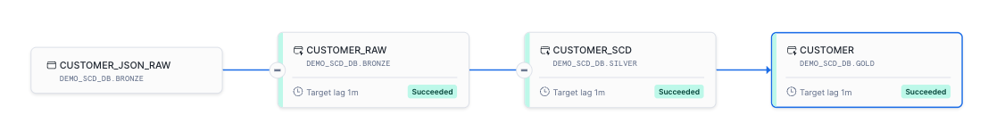
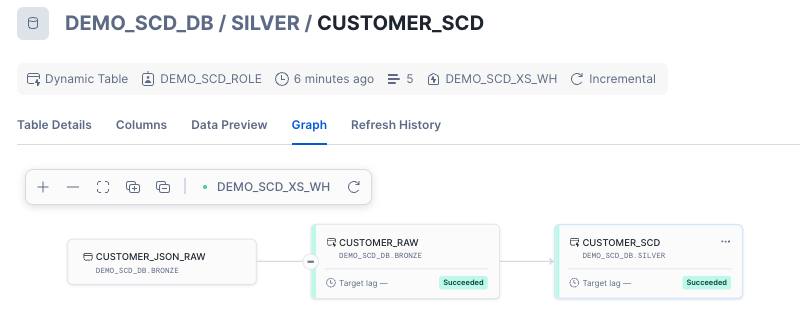
The graph above shows the dynamic table lineage from raw through gold. Because we set the target lag on the gold table to 1 minute and the lag on silver and bronze to downstream, Snowflake will automatically refresh the silver and bronze tables whenever the gold table needs refreshed. The 1 minute lag in this case is for demo purposes and under normal deployments, that lag should be set appropriately for your SLAs and data environment.
Why Dynamic Tables
For this simplified version of a real-world data engineering problem I encountered, dynamic tables eliminate the challenge of reloading out-of-order or late arriving data files. With the dynamic table pipeline in place, the files are simply loaded directly to the raw table and then the DAG handles the rest. Even further automation could be established through Snowpipe to auto ingest the files as they arrive, making this pipeline truly “hands off”.
Dynamic tables also simplify this workload in Snowflake. Prior to dynamic tables, this same pipeline could be established with Streams and Tasks; however, that would require creating a table, stream and task for each step in the process. Dynamic tables simplify that workload by creating one object for each step of the process. Streams and Tasks certainly still have their place in Snowflake pipelines – particularly when needing to call stored procedures within a data flow. Dynamic tables can’t do that at this time.
Wrap-Up
In this demo, we solved a real-world data engineering scenario using native Snowflake features and eliminated complexity for data engineers. First, we loaded JSON data directly to a VARIANT data column which then allows direct querying of the data. Next, we used JSON functions to flatten the data into a structured format using SQL and a dynamic table. Once the data was flattened, we used a second dynamic table to sort the data and display it as a SCD2 to track historical changes. Lastly, we created the driver dynamic table to store only the current record data from the SCD2 table.
The entire pipeline with dynamic tables eliminates the need for data engineers to setup complex methods of resetting and reloading SCD2 tables within the Snowflake Data Cloud. That allows them to shift focus from maintaining pipelines to building new ones and enriching data for the end-users, turning raw data into information to propel the business forward!
Follow me on LinkedIn and Medium for more data engineering and AI demos on Snowflake, Streamlit, and Python.

Good one but if possible, also do the video of this scenario by your own style
LikeLike